Best Model for the Data

It can be complicated to assess the best way to model data. How can you know if your model is good? How can you know what steps to take to make it better? Did you really make it better? In our exploration of these questions we will come across concepts such at interaction variables, residual plots, outliers, and collinearity.

I’m working with a csv file which I read into my R document and named ‘data2’. It contains 100 observations with the variables y, age, sexf, x1, x2, and x3. Our goal is to come up with a model that is very good at predicting y.

First, let’s look at how good the go-to regression is. That is, y regressed on all the independent variables.

two <- lm(y~ age + sexf + x1 + x2 +x3, data2)
summary(two)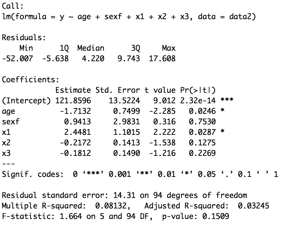

The Rsquared is .081 which is quite low indicating the model is not a good predictor of y. Let’s also note, we observe age and x1 to be the significant variables.

Step 1: Linearity

One of the fundamental assumptions of a linear model is the assumption that all variables are linear. Let’s check by looking at plots of all independent variables graphed against the residuals.

residuals <- resid(two)
plot(residuals~age,data2)
plot(residuals~sexf,data2)
plot(residuals~x1,data2)
plot(residuals~x2,data2)
plot(residuals~x3,data2)

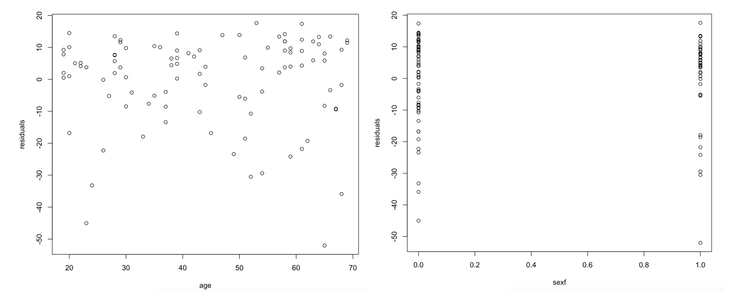
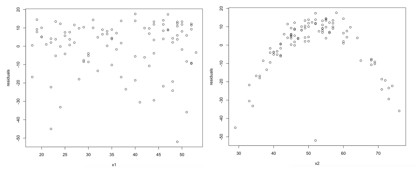
For the regression plots to be linear we want to see a random scatter of the observations. 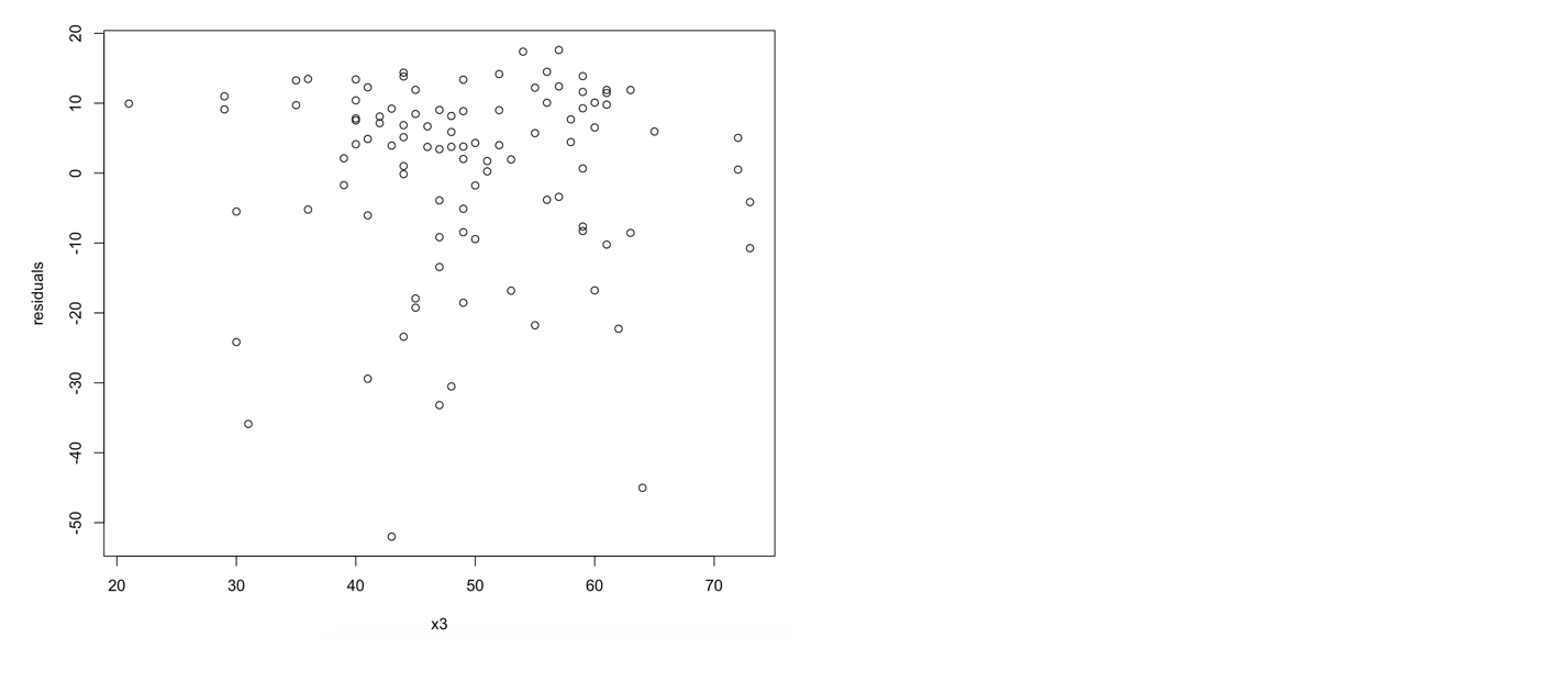The plots for age, x1, and x3 look random, so we can assume they are linear. The residual plot for sexf looks a bit different but is also random when we think about it. The variable for sex is either 0 or 1, so given that the observations can only be at those two marks on the axis we are really looking for a random spread on the y axis. And yes, there doesn’t appear to be a cluster of the data at any point of the y axis. Now finally we have the residual plot for x2. It appears to be following the trend of a negative parabola. This is a red flag that the x2 variable is nonlinear.

One way to compensate for this linearity problem is by adding another variable to the model that is the square of the nonlinear variable. To do this, I created a new column in our data set that is x2squared, then added that term in our regression. Additionally, I run a summary of our model so we can assess it.

data2$x22 <- data2$x2^2
three <- lm(y~ age + sexf + x1 + x2 +x3 + x22, data2)
summary(three)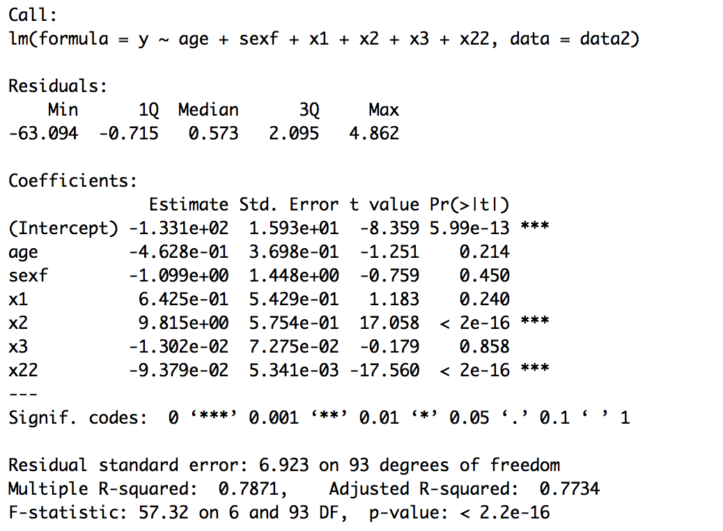

Our Rsquared value jumps to 0.787. This model is a much better fit than our previous model without the x2squared variable. Now we see that x2 and x2squared are the significant variables.

Step 2: Outliers

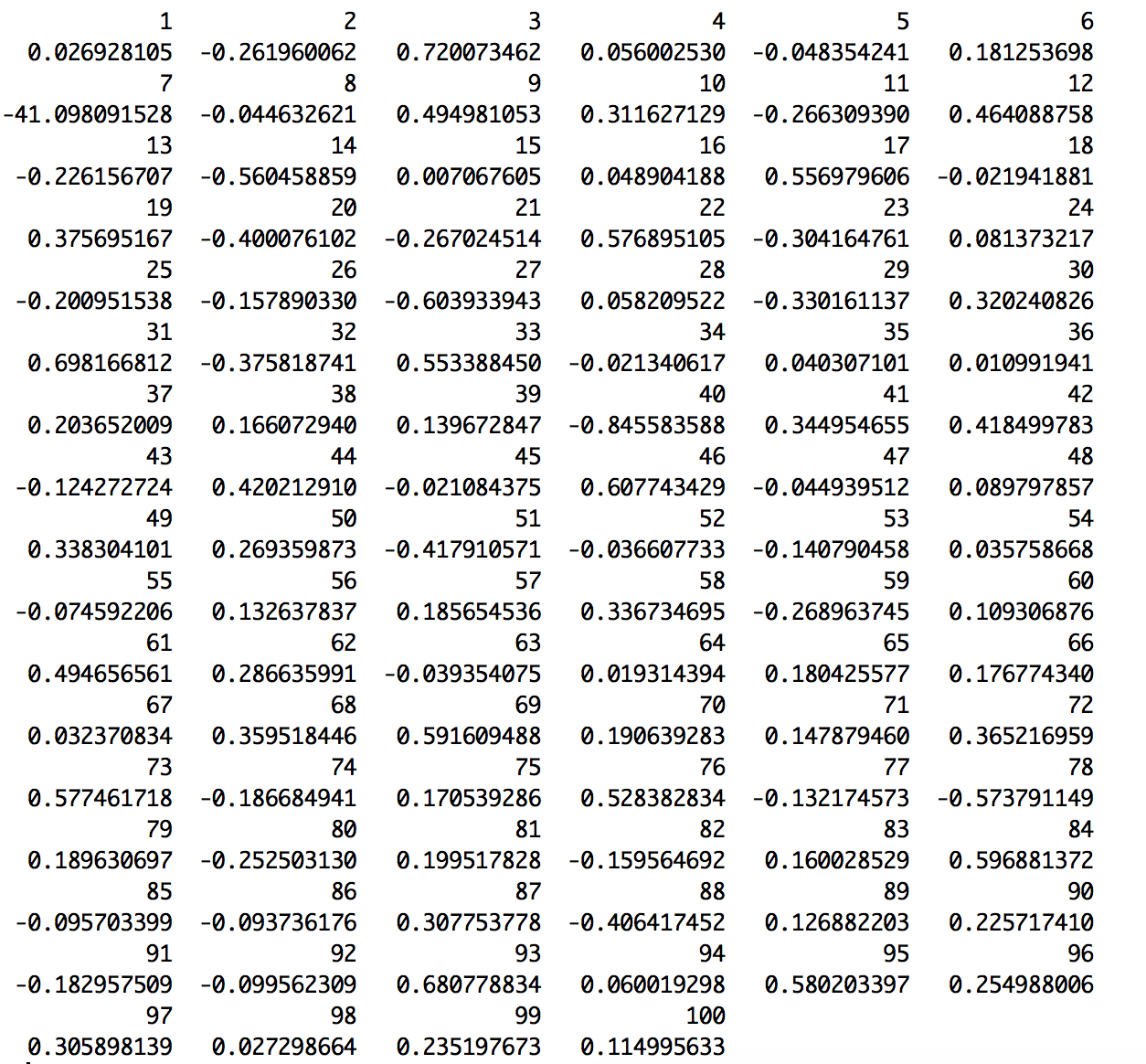
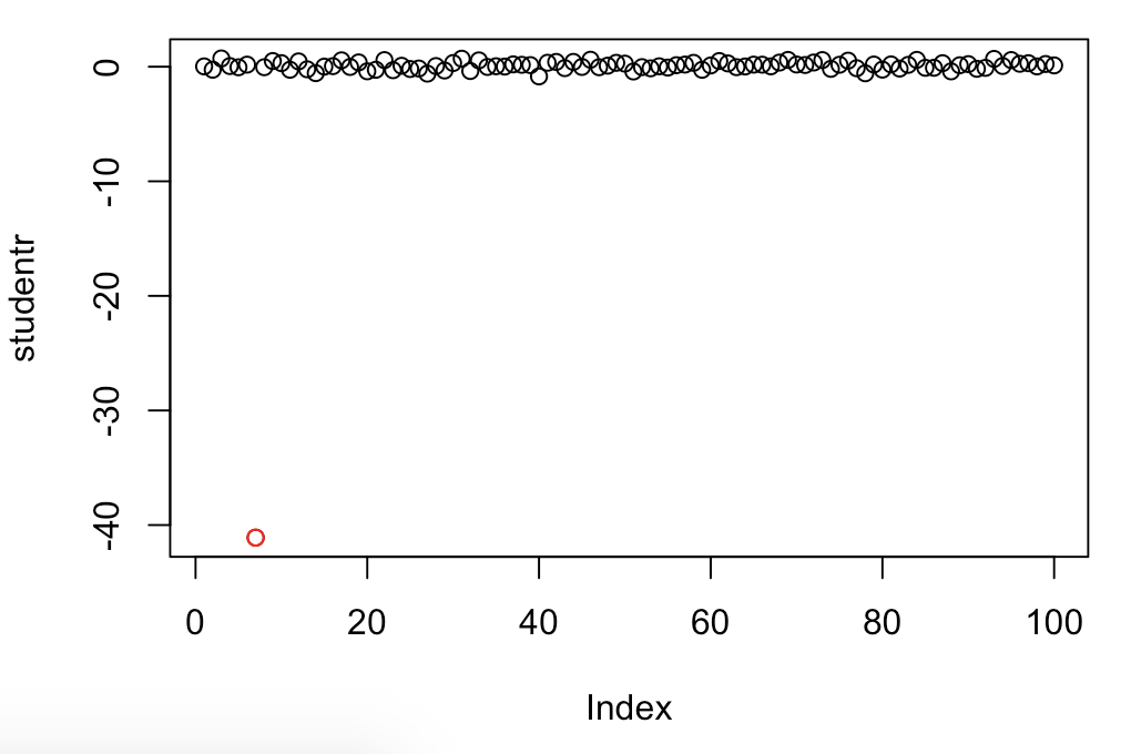
We can improve a model by checking for outliers and removing any we find significant. Let’s look at two criteria for determining outliers. The first is studentized residuals which follow a t table with n-k-1 degrees of freedom (n=sample size, k= number of regressor in model). In our case n=100 and k=6. our output will give us studentized residual values for each observation but these can be hard to read so, let’s also graph it.

studentr <- rstudent(three)
student r 
plot(studentr)
points(7,studentr[7],col="red")

It’s easy to see one point which is significant. I found the outlier point to be observation 7 because I could see it was around 10, then played around with coloring different observations on the graph until the outlier light up red. This was an easy way to get around searching through the list of numbers in the R output

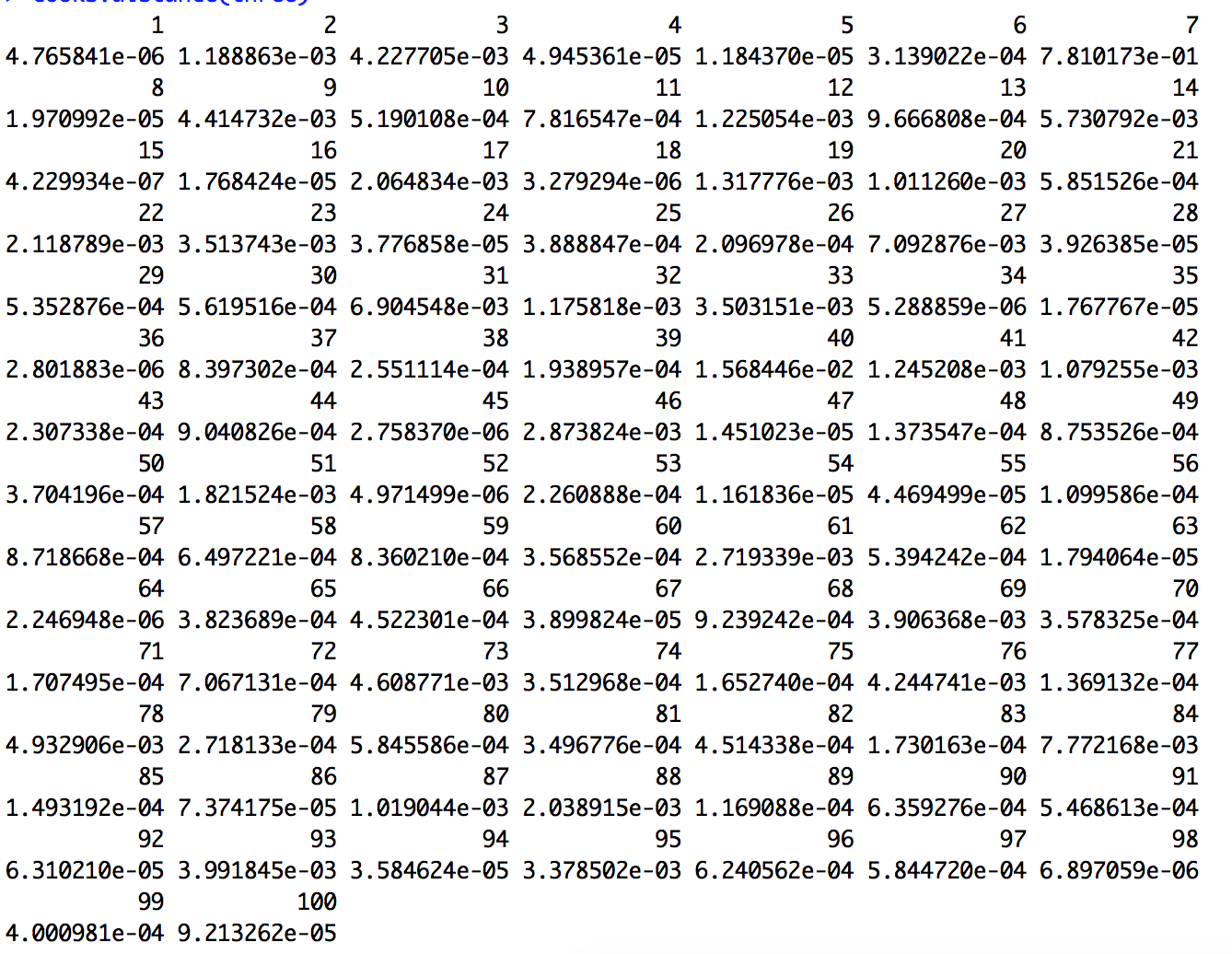
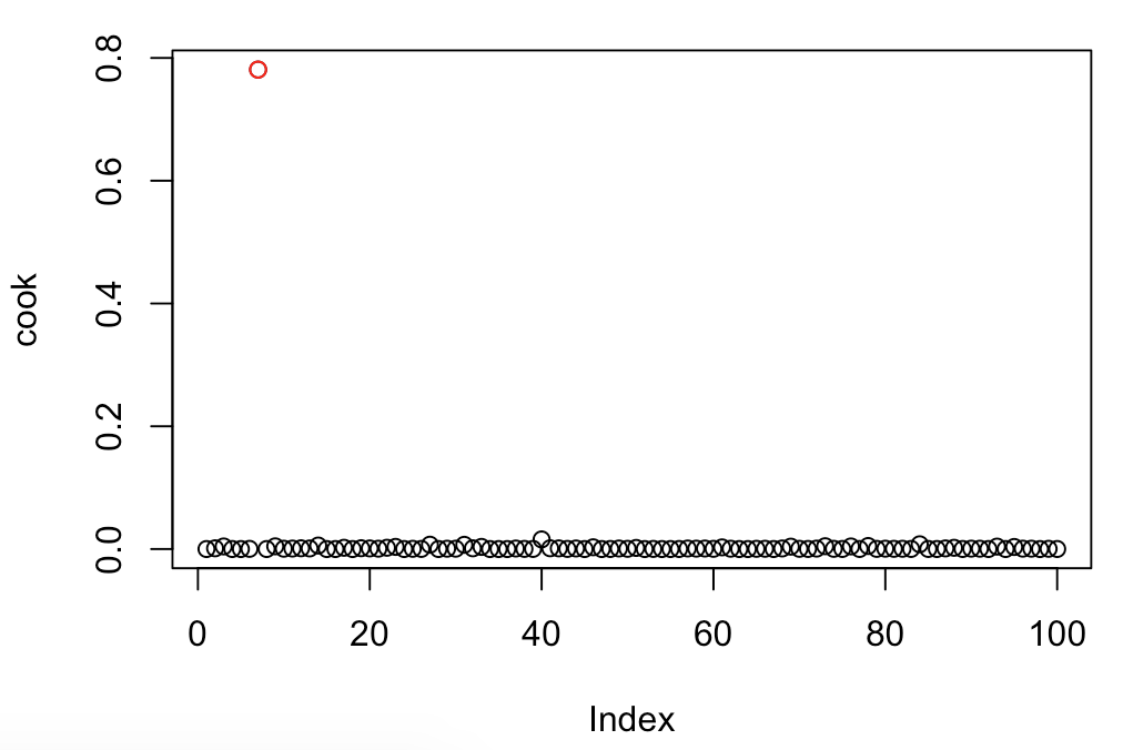
The second way to identify outliers is by calculating the Cook’s distance for each observation. Influential point for Cook’s distance will have a value greater than 4/n. In our case, we’re looking for values greater than 4/100 or .04.

cooks.distance(three)
cook <- cooks.distance(three)
plot(cook)
points(7,cook[7],col="red")

Similar to the studentized residuals we see observation 7 is an outlier.

After confirming observation 7 is an outlier the next step is to remove it. To do this we will be creating a new dataframe called ‘newdata’ which is a subset of our data. It will have all 8 of our variables but only 99 observations.

newdata <- data2[-c(7),]

Let’s see if removing the outlier improved our model

m <- lm(y~ age + sexf + x1 + x2 +x3 + x22, newdata)
summary(m)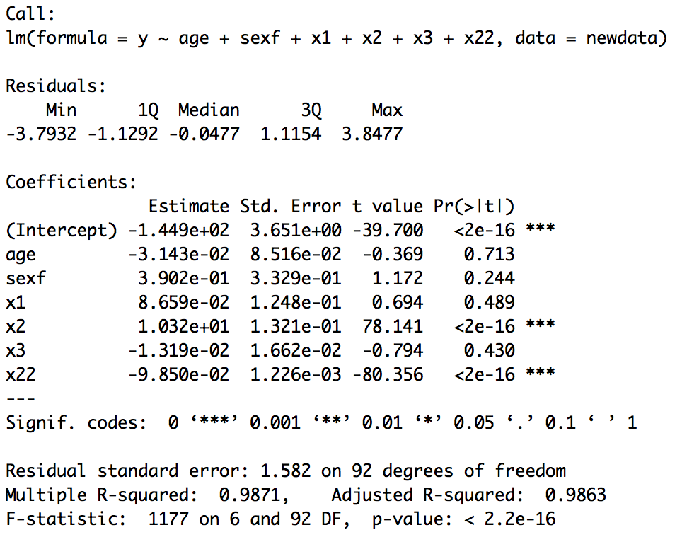

Yes, removing the outlier increase the Rsquared of the model to .9871 which is very high. We still see that only variables x2 and x2 squared are significant.

Step 3: Collinearity

Variance inflation factor(VIF) is a value assigned to each independent variable in a model to describe collinearity. A high VIF value means that variable is highly correlated with another variable in the model. We should expect that x2 and x2squared will have high VIF values because they are highly correlated. But, let’s check if any other variables in our model are correlated.

vif(m)

It appears age and x1 are also highly correlated. When two variables that are highly correlated are in the model it can create problems. Because both are present neither would seem like an important contribution. However, when one is not present the other may be highly significant. So, let’s remove x1 from our model and the updated model.

m5 <- lm(y~ age + sexf + x2 +x3 + x22, newdata)
summary(m5)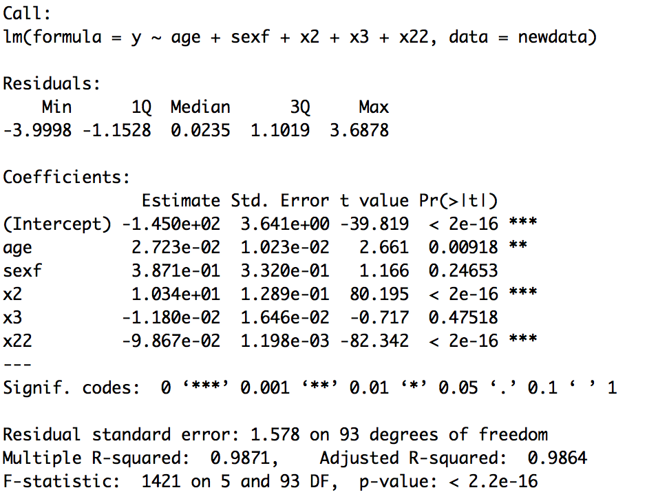

Our Rsquared value has stayed just as strong as before at .9871 so our model is good at predicting the data. The difference is now, x2 x2squared, and age are significant predictors. At this point we can be very satisfied with the model we have chosen to predict our data.