Choosing a Time Series Model

In this post I will look at common graphs to analyze a time series dataset covering topics such as stationarity, transformation, ACF plots, and PACF plots.

Let’s look at the dataset built in R called sunspot.year. It is a time series dataset that records the yearly number of sunspots from 1700 to 1988.

First, we should take a look at the data.

plot.ts(sunspot.year,ylab="Number of Sunspots")
title(main = "sunspots.year")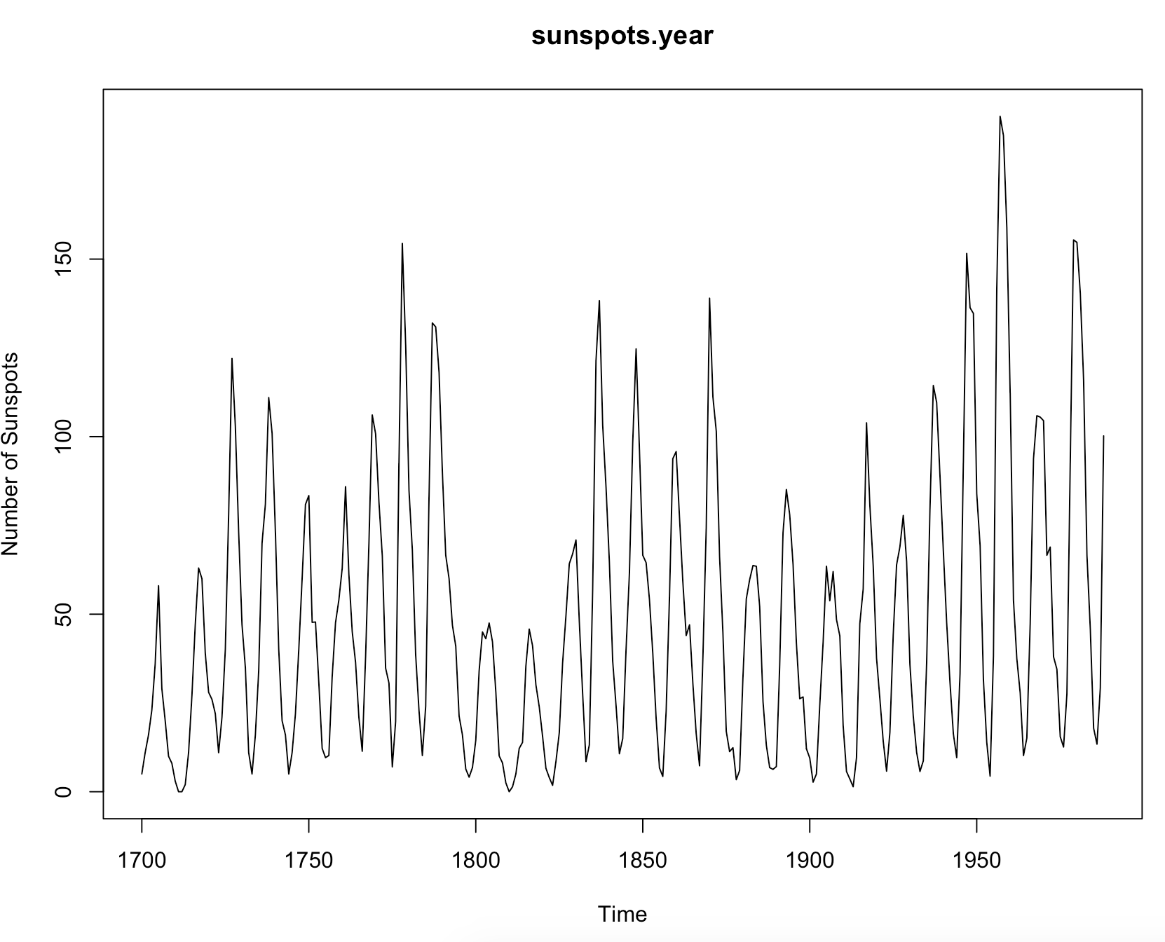

It looks like as the years go by, the average number of sunspots is increasing. In other words, there is a positive linear trend, which can also be preferred to as a non-constant mean. The variance also appears to be increasing over time. The non-constant mean and non-constant variance are both indicators that the data is non stationary.

Time series data needs to be made stationary before we can judge what model to fit the data with. A way to correct for a non-constant mean is to apply a square root transformation to the data. So, let’s do this and reassess the plotted data

newsunspot=sqrt(sunspot.year)
plot.ts(newsunspot, ylab= "Square Root Number of Sunspots")
title(main = "Transformed sunspots.year")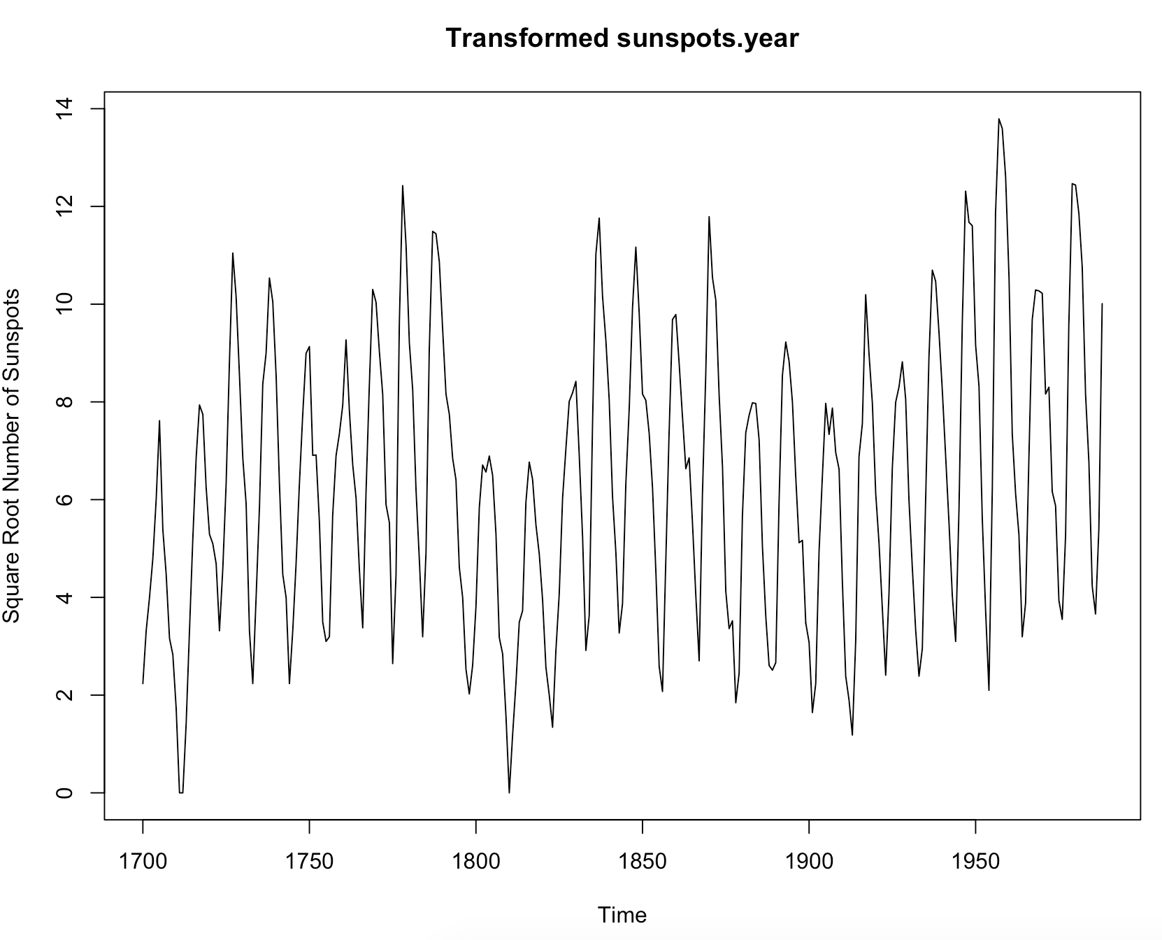

The transformed data now appears to have a constant variance around 6. Additionally, there are no obvious issues with the variance. The transformation was a success because the data now looks stationary.

Now that the data has been corrected to behave stationary, we can identify a model looking at the autocorrelation(ACF) and partial autocorrelation functions(PACF). Keep in mind only the ACF and PACF graphs obtained from the transformed data are useful because they have been corrected. Note, the first line of code displays the graphs side by side for convenience.

par(mfrow=c(1,2))
acf(newsunspot, main="Transformed sunspots.year")
pacf(newsunspot, main="Transformed sunspots.year")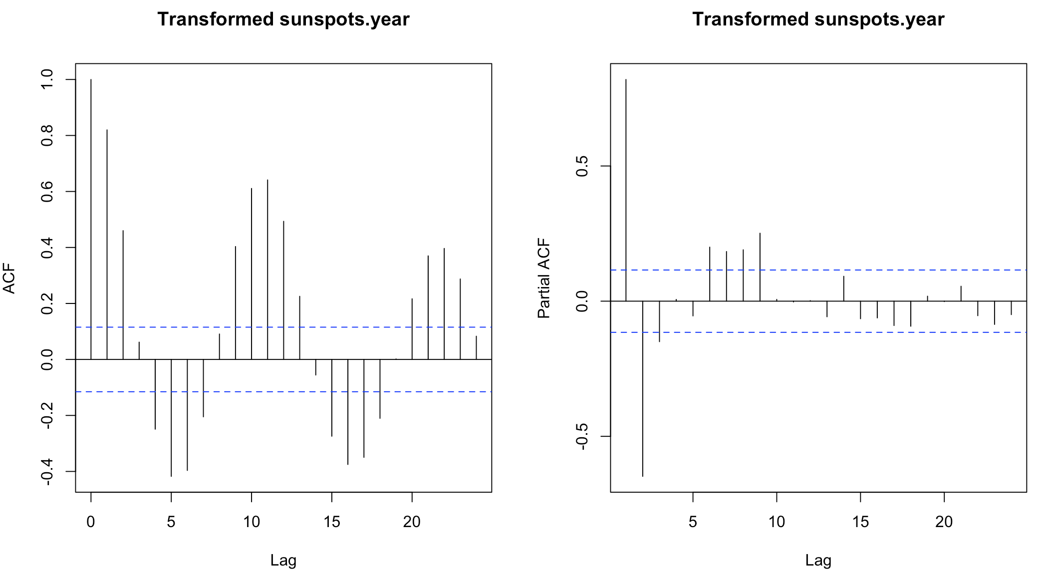

The ACF corrosponds to the MA (moving average) component of the model, while the PACF corrosponds to the AR (autoregressive) component. Models be composed of both components or just one.

When the ACF graph has all lags significant while decaying to zero, this indicates an MA(0) component. Likewise, if the PACF was significant at all lags and decaying to zero, this would indicate AR(0). If both decay to zero inthis manner it would suggest a lower order ARMA model. But here we believe an MA(0)compnent. The PACF of our data is highly significant at lag one and two but becomes insignificant at lag three onward. Because the PACF “cuts off” after lag 2 we believe an AR(2) component is the best fit.

So, in this case the graphs indicate that the data follows an ARMA(2,0) also expressed as AR(2).