Forecasting Time Series Data

Let’s look at the time series dataset in R called co2. This dataset measures monthly Mauna Loa atmospheric CO2 concentration from 1959 to 1997 totaling 468 observations.

We will be forecasting the data using three methods then comparing the methods of forecast. How do you compare methods or their accuracy? We will slip the data up into two parts. The first 1 thorough 444 observations will be called the training data. This is the portion of the data we will base our forecasting on. The last 5% of the data (i.e. the last 24 observations) is called the test data. The training data will be used to predict the last 24 observations, then predicted values and test data can be compared to measure accuracy of the model. For what we want to do we need additional packages. If you have never before worked with them, remember to install the packages before you can load them into your library.

library(TSA)
library(fArma)
library(forecast)
train <- co2[1:444]
test <- co2[445:468]

Let’s take a look at the data.

plot.ts(co2)
par(mfrow=c(1,2))
acf(co2)
pacf(co2)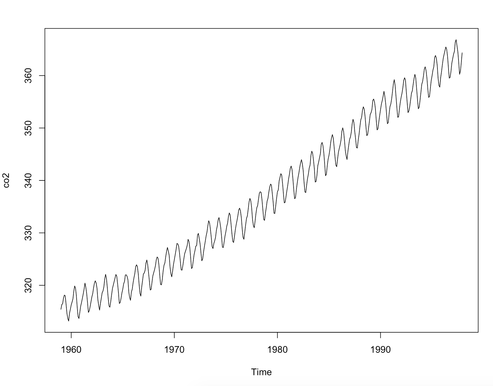

The time series data has a positive linear trend. There are no issues with heteroscedasticity. The constant up and down pattern indicates a seasonal trend of period 12.

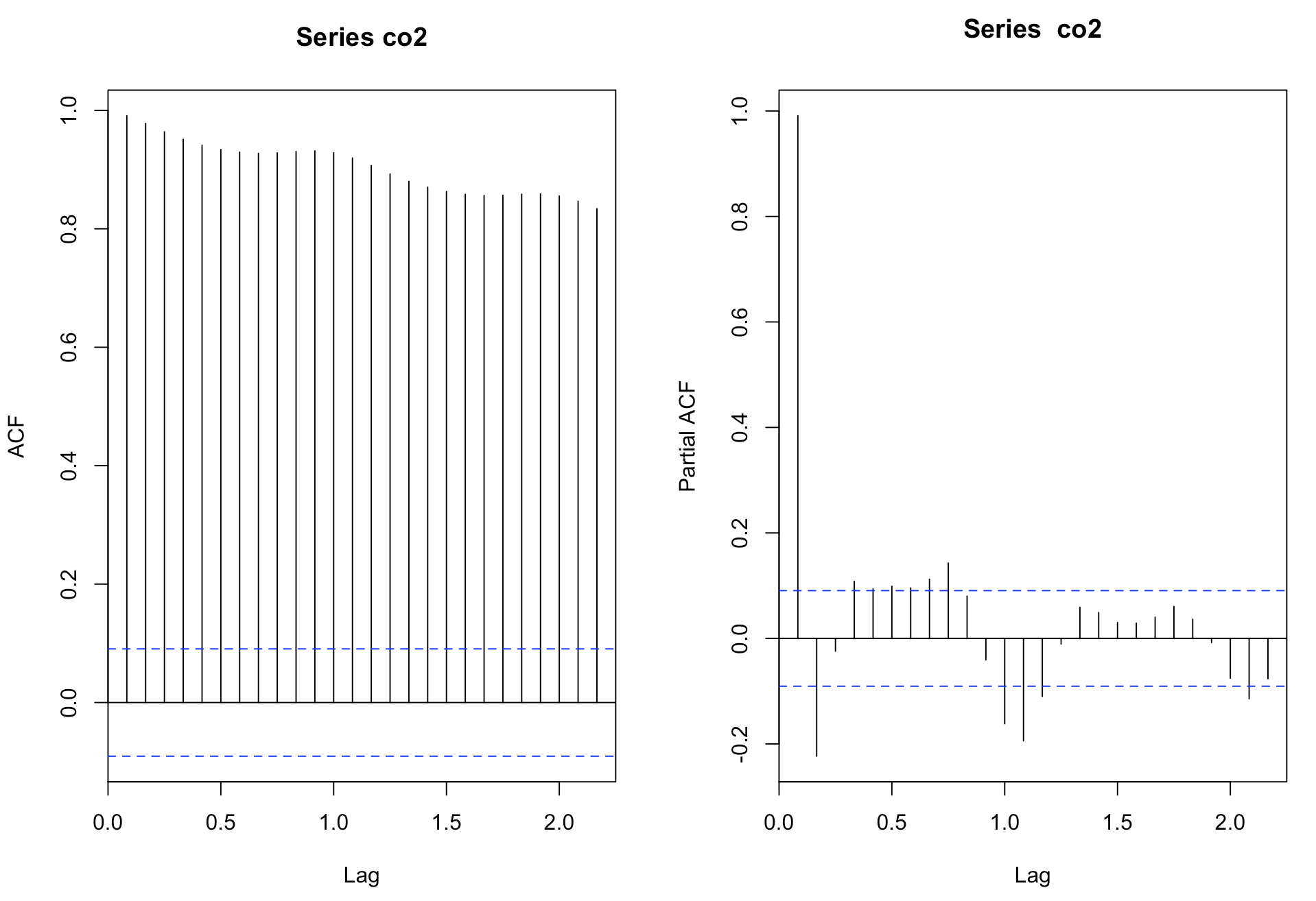This is a unique ACF PACF combination that indicates nonstationarity. The ACF decays to zero at a very slow rate while the PACF is only really significant at lag 1. We expected to see signs of nonstationarity because of the non-constant mean we previously noted.

Forecast 1

The first method of forecasting we will try is called subset selection method. This is a computer method where we input the maximum AR and MA orders we believe may explain the model, here we will choose 15 for both. The computer program then runs through all possible ARMA model combinations of those coefficients and returns the most probable models based on their BIC values.

sub1 <- armasubsets(diff(diff(train,12)),nar=15,nma=15)
plot(sub1)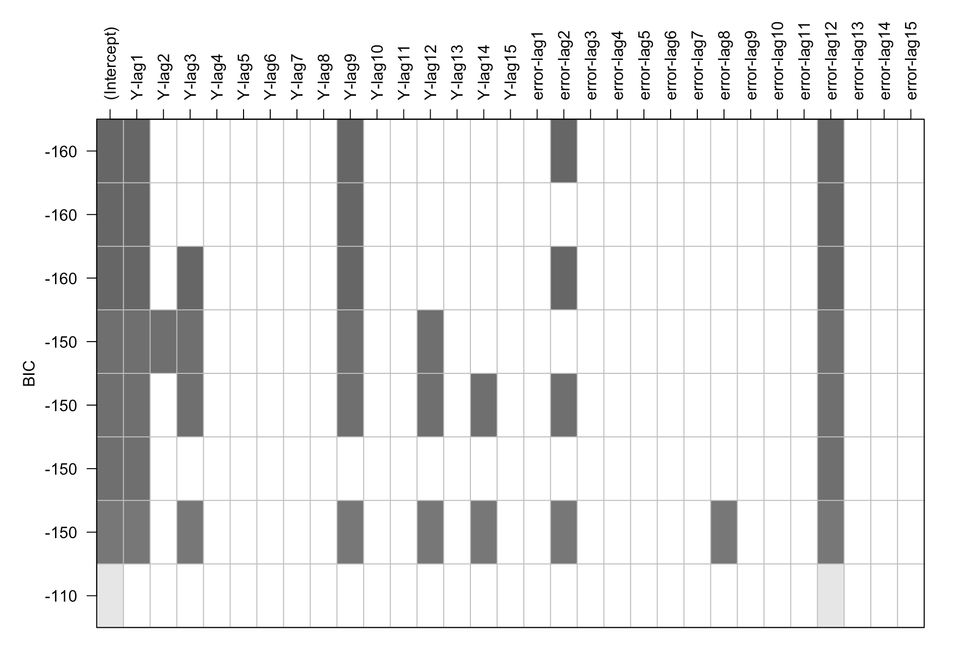

Based on our output, we believe the best model is an ARIMA(9,1,12). The 1 indicates that we applied a differencing to the data. The AR component is 9 because that is the highest order coefficient however there is also a nonzero coefficient value for phi 1. Similarly, the MA component is 12 because that is the highest order coefficient however there is also a nonzero coefficient value for theta 2. The Arima function below gives us the values for the coefficients of the ARIMA model.

arma1 <- Arima(train,order=c(9,1,12), seasonal=c(0,1,0),fixed=c(NA,rep(0,7),NA,0,NA,rep(0,9),NA))
arma1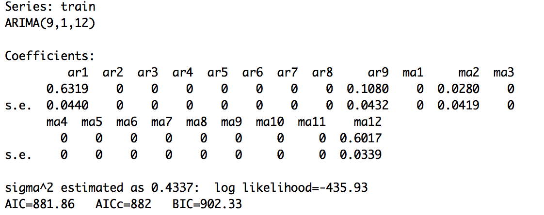

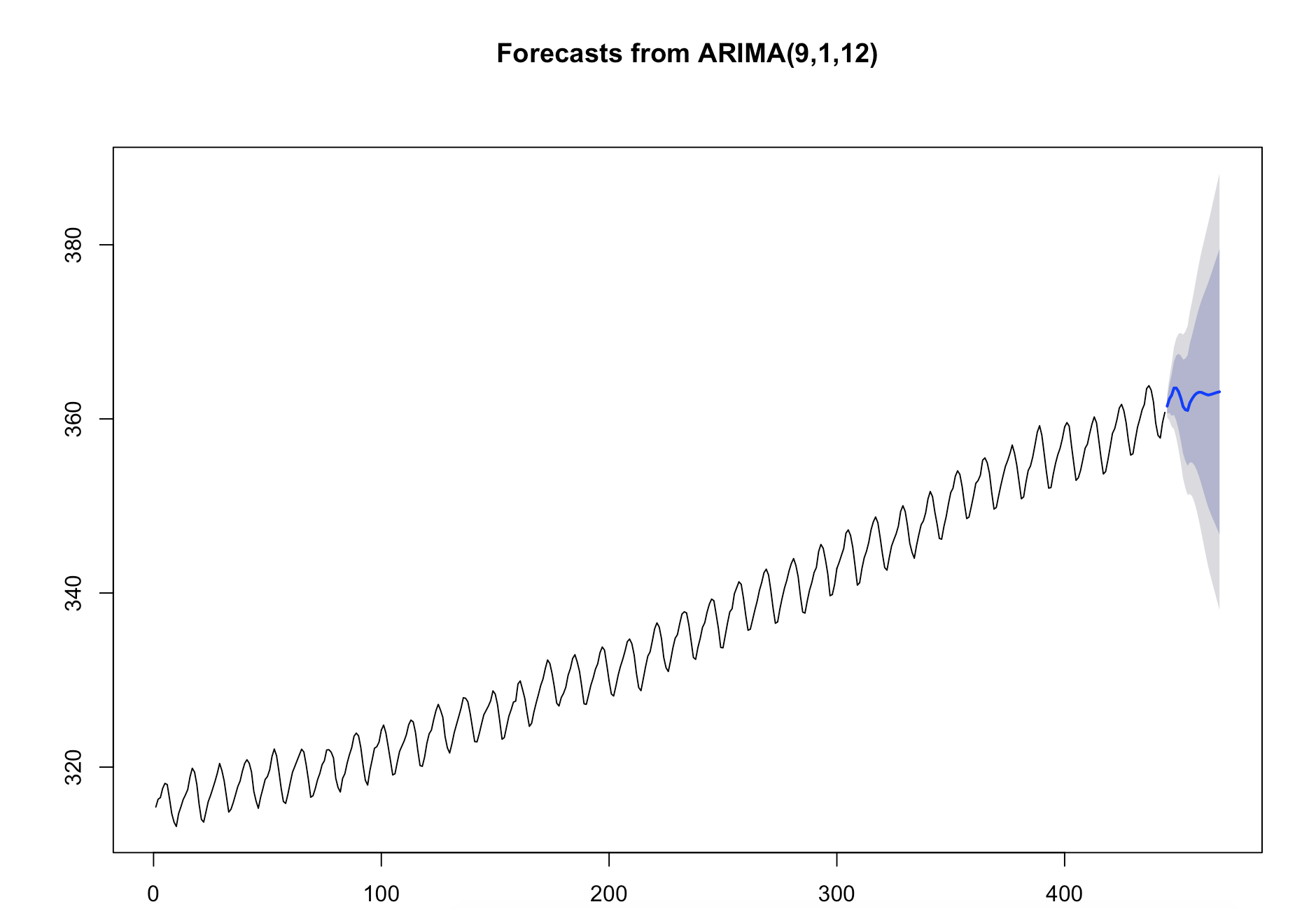
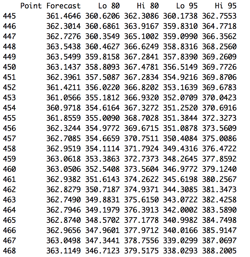
We can see below that the forecast isn’t doing a very good job at following the pattern of the data in the prediction. Additionally the confidence intervals are very large. While all of the test data points are in the respective confidence intervals, this model does not look ideal.

Forecast 2

The next method of forecasting will be to identify potential SARIMA models from the ACF and PACF. Then fit the candidate models and compare their AICc values to choose a final SARIMA model to run the forecast on.

We need to look at the ACF/PACF of the differenced data.

ddtrain <- diff(diff(train),12)
par(mfrow=c(1,2))
acf(ddtrain,lag.max=40,main="Differenced co2")
pacf(ddtrain,lag.max=40,main="Differenced co2")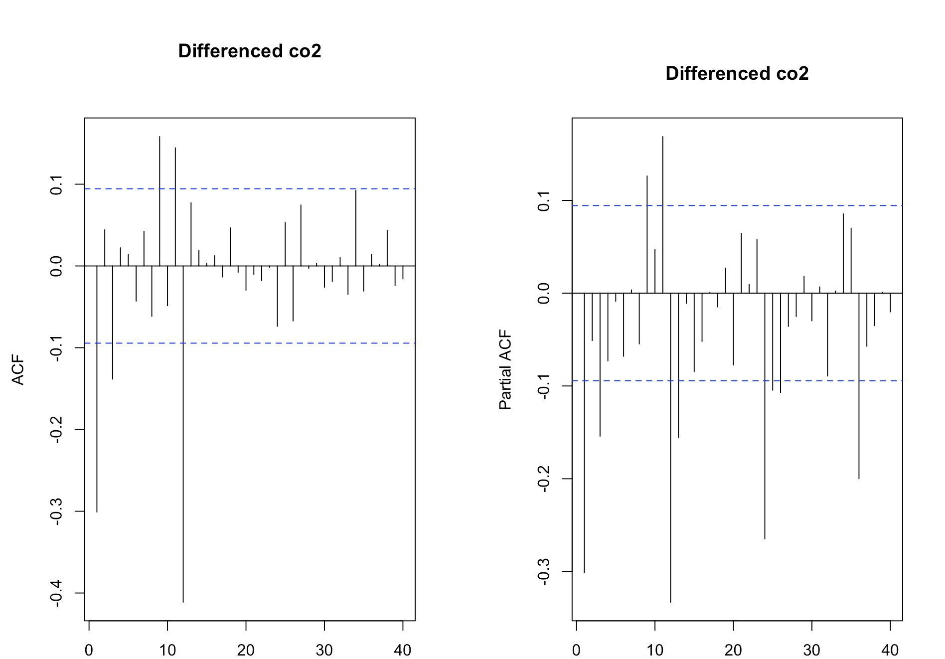

Both the ACF and PACF decay to zero for the first few lags which indicates that possible models could be AR(1) or MA(1) or ARMA(1,1). As for the seasonal component, the ACF cuts off after lag 1 (aka lag 12 but this is the first seasonal lag) and the PACF decays to zero at the seasonal lags (every twelfth lag). These suggest an MA(1) model is appropriate for the seasonal component.

Arima(ddtrain, order=c(0,1,1), seasonal=c(0,1,1))
Arima(ddtrain, order=c(1,1,0), seasonal=c(0,1,1))
Arima(ddtrain, order=c(1,1,1), seasonal=c(0,1,1))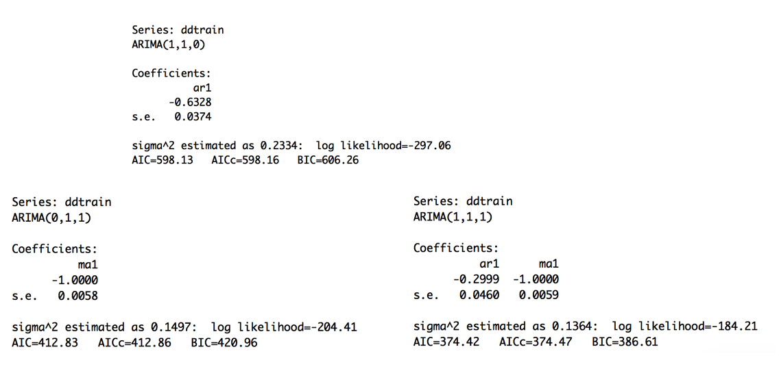

Of the three models we tested, SARIMA(1,1,1)x(0,1,1)[12] performed best with the lowest AICc value of 374.47. Below we see the model is not very good at predicting the testing data. The model does not keep the same seasonal pattern and is not even behaving in a positive linear manner. The confidence intervals are also very large.

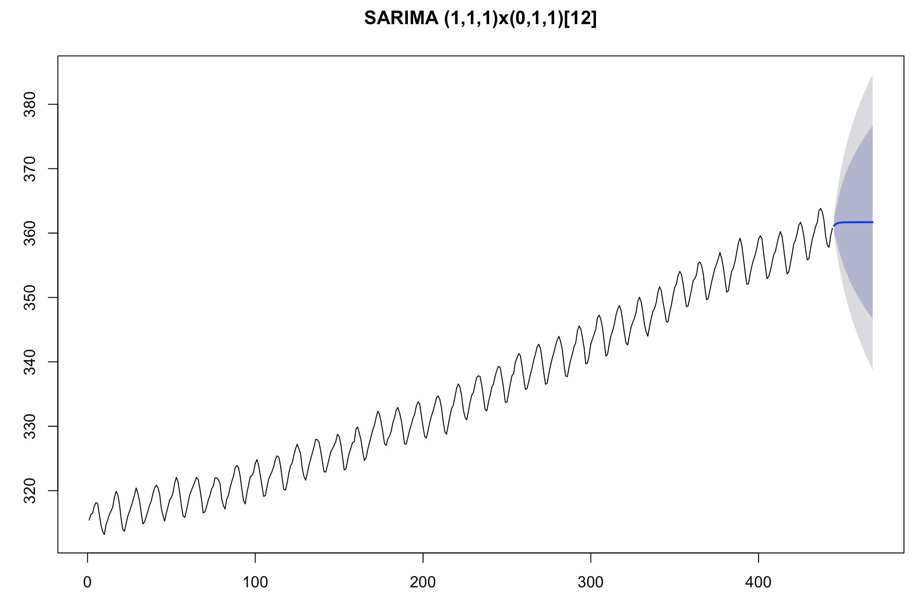
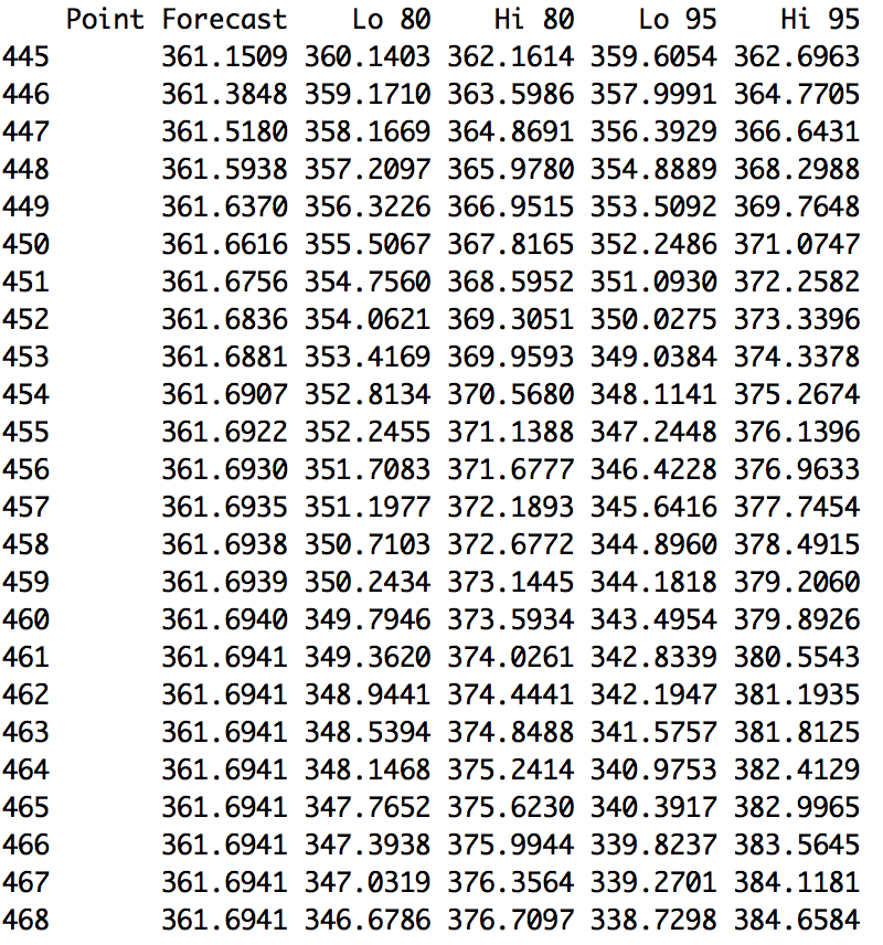
Forecast 3

The third method of forecasting is called a Holt-Winters seasonal forecast. We specify an additive seasonal trend instead of multiplicative because there is no heteroscedasticity. The “gamma = T” condition specifies that there is a seasonal component to address. The Holt-Winters is a form of double exponential smoothing that is good to use when there is a linear trend and/or a known seasonal component.

hw <- HoltWinters(ts(train,frequency=12),gamma = T, seasonal = "additive")
forecast(hw, h=24)
plot(forecast(x, h=24))

The Holt-Winters is a good predictor. The trend and seasonality patters are consistent with the previous data and the confidence intervals are narrow. Additionally, all 24 testing data points lie within the 95% prediction interval.

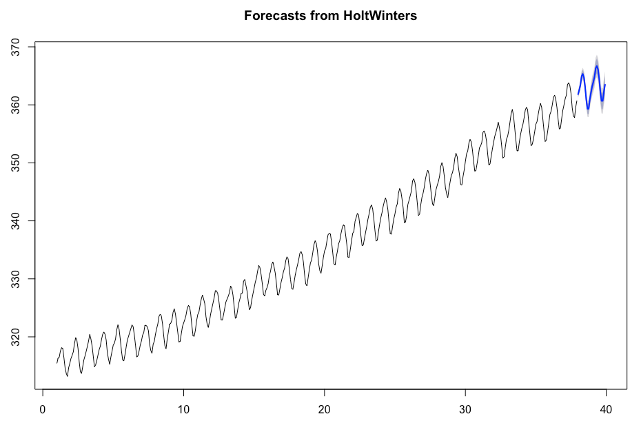
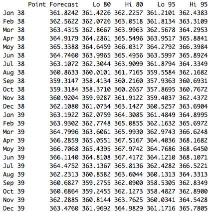
Comparing Forecastings

To compare the forecast, we will use two common criteria that quantify how much error the model produced. The lower the RMSE and MAPE the better the model was at predicting the testing data.

HWfcast1 <- forecast(arma1,h=24)
HWerr1 <- test-HWfcast1$mean
HWrmse1 <- sqrt(mean(HWerr1^2))
HWmape1 <- mean(abs((HWerr1*100)/test))
HWrmse1
HWmape1

ff2 <- Arima(train, order=c(1,1,1), seasonal=c(0,1,1))
HWfcast2 <- forecast(ff2,h=24)
HWerr2 <- test-HWfcast2$mean
HWrmse2 <- sqrt(mean(HWerr2^2))
HWmape2 <- mean(abs((HWerr2*100)/test))
HWrmse2
HWmape2

ff3 <- HoltWinters(ts(train,frequency=12),gamma = TRUE,seasonal="additive")
HWfcast3 <- forecast(ff3,h=24)
HWerr3 <- test-HWfcast3$mean
HWrmse3 <- sqrt(mean(HWerr3^2))
HWmape3 <- mean(abs((HWerr3*100)/test))
HWrmse3
HWmape3

As we expected the Holt- Winters forecasting was the best. Next, the ARIMA(9,1,12) model performed slightly better than the SARIMA(1,1,1)x(0,1,1)[12] model. A second look at the forecasting graphs for these two models confirms their performances. The SARIMA model had no trend or seasonal pattern while the ARIMA model did have a slight seasonal pattern in its prediction.